BMJ  2004;328:1073 (1 May), doi:10.1136/bmj.328.7447.1073

Education and debate

Statistics Notes

The logrank test

¹ Department of Health Sciences, University of York, York YO10 5DD, ² Cancer Research UK/NHS Centre for Statistics in Medicine, Institute of Health Sciences, Oxford OX3 7LF

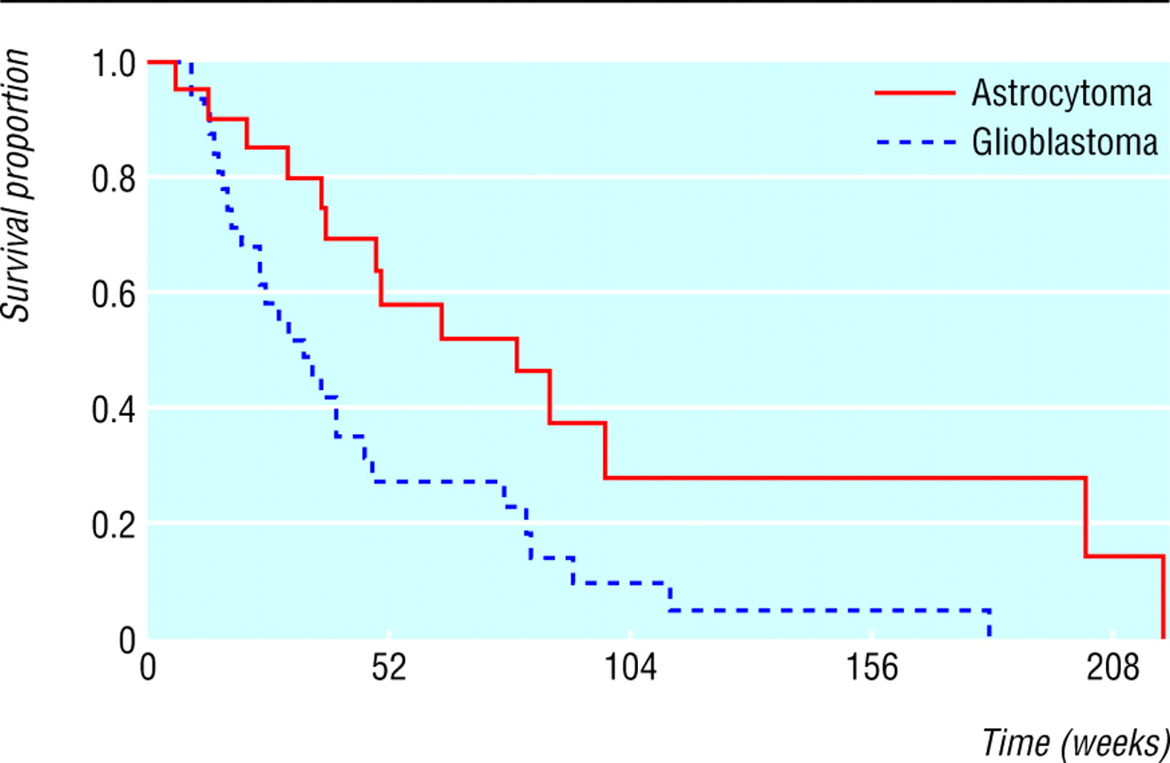
We often wish to compare the survival experience of two (or more) groups of individuals. For example, the table shows survival times of 51 adult patients with recurrent malignant gliomas¹ tabulated by type of tumour and indicating whether the patient had died or was still alive at analysis—that is, their survival time was censored.² As the figure shows, the survival curves differ, but is this sufficient to conclude that in the population patients with anaplastic astrocytoma have worse survival than patients with glioblastoma?

View this table: [in this window] [in a new window]   Weeks to death or censoring in 51 adults with recurrent gliomas1 (A=astrocytoma, G=glioblastoma)

 

View larger version (20K): [in this window] [in a new window]   Survival curves for women with glioma by diagnosis

 

We could compute survival curves³ for each group and compare the proportions surviving at any specific time. The weakness of this approach is that it does not provide a comparison of the total survival experience of the two groups, but rather gives a comparison at some arbitrary time point(s). In the figure the difference in survival is greater at some times than others and eventually becomes zero. We describe here the logrank test, the most popular method of comparing the survival of groups, which takes the whole follow up period into account. It has the considerable advantage that it does not require us to know anything about the shape of the survival curve or the distribution of survival times.

The logrank test is used to test the null hypothesis that there is no difference between the populations in the probability of an event (here a death) at any time point. The analysis is based on the times of events (here deaths). For each such time we calculate the observed number of deaths in each group and the number expected if there were in reality no difference between the groups. The first death was in week 6, when one patient in group 1 died. At the start of this week, there were 51 subjects alive in total, so the risk of death in this week was 1/51. There were 20 patients in group 1, so, if the null hypothesis were true, the expected number of deaths in group 1 is 20 x 1/51 = 0.39. Likewise, in group 2 the expected number of deaths is 31 x 1/51 = 0.61. The second event occurred in week 10, when there were two deaths. There were now 19 and 31 patients at risk (alive) in the two groups, one having died in week 6, so the probability of death in week 10 was 2/50. The expected numbers of deaths were 19 x 2/50 = 0.76 and 31 x 2/50 = 1.24 respectively.

The same calculations are performed each time an event occurs. If a survival time is censored, that individual is considered to be at risk of dying in the week of the censoring but not in subsequent weeks. This way of handling censored observations is the same as for the Kaplan-Meier survival curve.³

From the calculations for each time of death, the total numbers of expected deaths were 22.48 in group 1 and 19.52 in group 2, and the observed numbers of deaths were 14 and 28. We can now use a ² test of the null hypothesis. The test statistic is the sum of (O - E)²/E for each group, where O and E are the totals of the observed and expected events. Here (14 - 22.48)² / 22.48 + (28 - 19.52)² / 19.52 = 6.88. The degrees of freedom are the number of groups minus one, i.e. 2 - 1 = 1. From a table of the ² distribution we get P < 0.01, so that the difference between the groups is statistically significant. There is a different method of calculating the test statistic,⁴ but we prefer this approach as it extends easily to several groups. It is also possible to test for a trend in survival across ordered groups.⁴ Although we have shown how the calculation is made, we strongly recommend the use of statistical software.

The logrank test is based on the same assumptions as the Kaplan Meier survival curve³—namely, that censoring is unrelated to prognosis, the survival probabilities are the same for subjects recruited early and late in the study, and the events happened at the times specified. Deviations from these assumptions matter most if they are satisfied differently in the groups being compared, for example if censoring is more likely in one group than another.

The logrank test is most likely to detect a difference between groups when the risk of an event is consistently greater for one group than another. It is unlikely to detect a difference when survival curves cross, as can happen when comparing a medical with a surgical intervention. When analysing survival data, the survival curves should always be plotted.

Because the logrank test is purely a test of significance it cannot provide an estimate of the size of the difference between the groups or a confidence interval. For these we must make some assumptions about the data. Common methods use the hazard ratio, including the Cox proportional hazards model, which we shall describe in a future Statistics Note.

---

Competing interests: None declared.

References

1. Rostomily RC, Spence AM, Duong D, McCormick K, Bland M, Berger MS. Multimodality management of recurrent adult malignant gliomas: results of a phase II multiagent chemotherapy study and analysis of cytoreductive surgery. Neurosurgery 1994;35: 378-8.[ISI][Medline]
2. Altman DG, Bland JM. Time to event (survival) data. BMJ 1998;317: 468-9.[Free Full Text]
3. Bland JM, Altman DG. Survival probabilities. The Kaplan-Meier method. BMJ 1998;317: 1572.[Free Full Text]
4. Altman DG. Practical statistics for medical research. London: Chapman & Hall, 1991: 371-5.

CiteULike    Complore    Connotea    Del.icio.us    Digg    Reddit    Technorati    What's this?

This article has been cited by other articles:

• O'Kelly, C., Macdonald, R. L. (2008). Coiling and Aneurysm Rerupture: Incomplete Treatment Is a Causal Intermediate Not a Confounder. Stroke 39: e121-e121 [Full text]  
• Malenka, D. J., Kaplan, A. V., Lucas, F. L., Sharp, S. M., Skinner, J. S. (2008). Outcomes Following Coronary Stenting in the Era of Bare-Metal vs the Era of Drug-Eluting Stents. JAMA 299: 2868-2876 [Abstract] [Full text]  
• Ajani, J. A. (2008). In Reply. JCO 26: 2236-2237 [Full text]  
• Escrig, R., Arruza, L., Izquierdo, I., Villar, G., Saenz, P., Gimeno, A., Moro, M., Vento, M. (2008). Achievement of Targeted Saturation Values in Extremely Low Gestational Age Neonates Resuscitated With Low or High Oxygen Concentrations: A Prospective, Randomized Trial. Pediatrics 121: 875-881 [Abstract] [Full text]  
• Cheang, M. C.U., Voduc, D., Bajdik, C., Leung, S., McKinney, S., Chia, S. K., Perou, C. M., Nielsen, T. O. (2008). Basal-Like Breast Cancer Defined by Five Biomarkers Has Superior Prognostic Value than Triple-Negative Phenotype. Clin. Cancer Res. 14: 1368-1376 [Abstract] [Full text]  
• Linden, T., Gerss, J., Jurgens, H. (2007). The crux of the log rank test. Re: Locasciulli A, Oneto R, Bacigalupo A, Socie G, Korthof E, Bekassy A, Schrezenmeier H, Passweg J, Fuhrer M. Outcome of patients with acquired aplastic anemia given first line bone marrow transplantation or immunosuppressive treatment in the last decade: a report from the European Group for Blood and Marrow Transplantation. Haematologica 2007; 92:11-8. haematol 92: e122-e122 [Full text]  
• Du, Y., Cullum, I., Illidge, T. M., Ell, P. J. (2007). Fusion of Metabolic Function and Morphology: Sequential [18F]Fluorodeoxyglucose Positron-Emission Tomography/Computed Tomography Studies Yield New Insights Into the Natural History of Bone Metastases in Breast Cancer. JCO 25: 3440-3447 [Abstract] [Full text]  
• Onate-Ocana, L. F., Milan-Revollo, G., Aiello-Crocifoglio, V., Carrillo, J. F., Gallardo-Rincon, D., Brom-Valladares, R., Herrera-Goepfert, R., Duenas-Gonzalez, A. (2007). Treatment of the Adenocarcinoma of the Esophagogastric Junction at a Single Institution in Mexico. Ann. Surg. Oncol. 14: 1439-1448 [Abstract] [Full text]  
• Ojha, R.P., Prabhakar, D., Evans, E., Lowery, K., Thertulien, R., Fischbach, L.A. (2007). RE: Abou-Jawde et al. The role of race, socioeconomic status, and distance traveled on the outcome of African-American patients with multiple myeloma. haematol 92: e46-e46 [Full text]  
• Onate-Ocana, L. F., Aiello-Crocifoglio, V., Gallardo-Rincon, D., Herrera-Goepfert, R., Brom-Valladares, R., Carrillo, J. F., Cervera, E., Mohar-Betancourt, A. (2007). Serum Albumin as a Significant Prognostic Factor for Patients with Gastric Carcinoma. Ann. Surg. Oncol. 14: 381-389 [Abstract] [Full text]  
• Chan, J. K., Cheung, M. K., Husain, A., Teng, N. N., West, D., Whittemore, A. S., Berek, J. S., Osann, K. (2006). Patterns and Progress in Ovarian Cancer Over 14 Years.. Obstet Gynecol 108: 521-528 [Abstract] [Full text]  
• Carey, L. A., Perou, C. M., Livasy, C. A., Dressler, L. G., Cowan, D., Conway, K., Karaca, G., Troester, M. A., Tse, C. K., Edmiston, S., Deming, S. L., Geradts, J., Cheang, M. C. U., Nielsen, T. O., Moorman, P. G., Earp, H. S., Millikan, R. C. (2006). Race, breast cancer subtypes, and survival in the Carolina Breast Cancer Study.. JAMA 295: 2492-2502 [Abstract] [Full text]  
• Grabenbauer, G. G., Lahmer, G., Distel, L., Niedobitek, G. (2006). Tumor-Infiltrating Cytotoxic T Cells but not Regulatory T Cells Predict Outcome in Anal Squamous Cell Carcinoma.. Clin. Cancer Res. 12: 3355-3360 [Abstract] [Full text]  
• Collantes-Fernandez, E., Lopez-Perez, I., Alvarez-Garcia, G., Ortega-Mora, L. M. (2006). Temporal Distribution and Parasite Load Kinetics in Blood and Tissues during Neospora caninum Infection in Mice. Infect. Immun. 74: 2491-2494 [Abstract] [Full text]  

Rapid Responses:

Read all Rapid Responses

Typographical error

J Martin Bland
bmj.com, 30 Apr 2004 [Full text]

Am I missing something?

Habab Rashid
bmj.com, 5 May 2004 [Full text]

Yes : you missed 'typographical error' !

L S Lewis
bmj.com, 6 May 2004 [Full text]

Two sided test use should be emphasised in medicine

Alan C Gibbs
bmj.com, 10 May 2004 [Full text]

Re: Two sided test use should be emphasised in medicine

J Martin Bland
bmj.com, 13 May 2004 [Full text]